Writing and Using Functions

In this chapter, we discuss functions.

Why use functions?
Creating Functions
Editor
Calling Functions
Comments
Multiple Functions Per File
Nesting Functions
Recursive Functions
Function Handles / Anonymous Functions
Function composition
Variable number of Input Arguments
Variable number of Output Arguments
Matlab path

Why use functions?

While we can perform a lot by simply writing script files or executing commands at the command prompt, there are many reasons why writing functions to perform computations and actions is advantageous. Many of these reasons would be discussed in a general course on programming. We simply list a few reasons here.

We can parameterize functions to call them multiple times with different inputs, instead of repeating the same code with different values plugged in.
We can compose functions together, and pass functions to other functions.
Functional code is often better organized, and easier to read and understand.
Variables inside a function only exist inside the function, so we can reuse the same variable name multiple times. (This is called lexical scoping.)
In Matlab, executing functions is faster than executing scripts.

Creating Functions

To create your own function, open a new file in the editor by typing edit filename.m and begin by creating the function header, which includes the name of the function and its inputs and outputs. When you save the m-file, you should give it exactly the same name as the function name in the header. (If there is a conflict between the filename and function name, the filename wins; however, the matlab editor will give a warning about any such inconsistency.) You cannot create functions within script files (except for anonymous functions discussed below).

function [output1 ,output2, output3] = myfunction(input1, input2)

Within the function, you can use the inputs as local variables and you must assign values to each of the outputs before the function terminates, (at least those that will be assigned by the caller of the function). It is customary to end the function with the end keyword but this is optional unless you have nested functions or multiple functions per file as described below.

Here is an example of a simple function. It must be saved in a file called quadform.m.

function [X1,X2] = quadform(A,B,C)
% Implementation of the quadratic formula.
% Here A,B and C can be matrices.
    tmp = sqrt(B.^2 - 4*A.*C);
    X1 = (-B + tmp)./(2*A);
    X2 = (-B - tmp)./(2*A);
end

We can call this as follows

[X1,X2] = quadform(1,10,3)

X1 =
   -0.3096
X2 =
   -9.6904

Editor

As we mentioned, Matlab commands are executed either at the command prompt or by running scripts or functions, which can be created and edited with the built in editor. To launch the editor, if it is not already open, type edit or edit filename. Commands can be entered here and executed as a script. They are saved with a .m extension. To run your script, type in the name at the command prompt, or press F5 or the save and run button at the top of the editor. Your own functions can be written here as well, as discussed here. You can set break points to halt execution at certain lines for debugging, which we discuss here.

Expressions that are too long for one line can be broken across lines by adding ... to the end of each line.

Comments are written by preceding the line with the % symbol. Block comments are opened with %{ and closed with %}. To have Matlab word wrap a selection of comments, right click on the highlighted text and select, Wrap Selected Text.

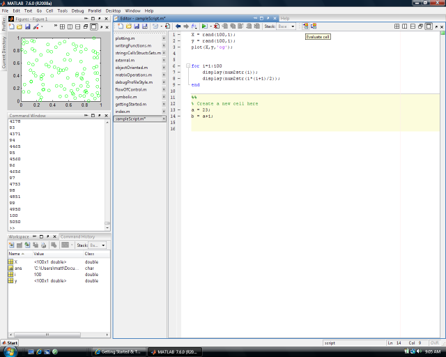
You can partition your code into editor cells by typing two percent signs, %%, at the beginning of the line. This can help organize your code into logical sections. You can also evaluate cells one at a time by selecting the evaluate cell button at the top of the editor. At any time, you can execute an arbitrary block of code by highlighting it and pressing F9. Cells are also used when publishing your code. This tutorial was written in Matlab and published to html by selecting the publish button at the top of the editor. This can be very useful when you want to share your code and results with others in a professional looking report.

Certain constructs like for loops and functions can be folded, hiding all but the top line from view. Select the + or - symbols appearing on the left hand side of the editor, by the line numbers.

Here is an image of the editor in action. Notice we have the open m-files listed in the center column; you can move these to the left right or bottom. We have also docked one of the figures in the top left. By default figures open in their own windows but it can sometimes be useful to work with a figure on the same screen: to do this, use the doc window arrow at the the top left of the figure.

There are many other configuration options and editor tools available; experiment by selecting the many buttons and exploring the drop down menus.

Matlab gives you a lot of freedom over how you organize the windows in the environment. For instance, you can have have multiple windows take up the same screen area and toggle between them at will, or place windows at the sides where they automatically hide until you select them. Try dragging them around to different places to see the effect. There are more windows than described here available under the Desktop drop down menu.

You can save the current layout, select one of the default ones, tile all the windows, and perform many other related tasks under the Desktop drop down menu. Its worth taking the time to organize your layout effectively before you begin working.

Calling Functions

We call a function we have written just like any other built-in matlab function. However, some functions can be executed as 'infix' operators like '+', or with their own special syntax as with the concatenation function, [ ]. In these last two cases, the special syntax is a kind of shorthand for the execution of the underlying function: 'a+b' executes plus(a,b) and '[a b]' executes horzcat(a,b) .

A = plus(2,2)                           % call the plus function
B = 2+2                                 % infix call to plus
nums = [1 3 4 2 8 4 3 1 9 2 3 1 3];     % call to the horzcat function

Note that functions may return any number of outputs, including 0, and may take any number of inputs, including 0. When a function takes no arguments, the use of parentheses is optional as in version or version(). If we do not supply any names to the outputs of a function and it returns outputs, the first, and only the first, of those outputs is assigned to the ans variable. In general, if a function returns n values, we can assign 0 to n of those by supplying 0 to n variable names enclosed in square brackets as in the examples below.

version                                % use of () optional if no arguments
unique(nums)                            % output assigned to 'ans'
C = unique(nums);                       % grab only the first of three outputs
[C,D] = unique(nums);                   % grab the first two
[C,D,E] = unique(nums);                 % grab all three

ans =
7.10.0.499 (R2010a)
ans =
     1     2     3     4     8     9

When a function takes only string arguments, we can call it using command syntax as in the following examples. Each input is separated by a space.

display hello                           % command syntax
strcat one two three four               % four inputs

hello
ans =
onetwothreefour

Matlab uses call-by-value semantics, meaning that (conceptually) all arguments are copied into the formal parameters of the function. That is, call-by-reference (pointers) is not used (although Matlab does have a new handle class that can implement this kind of mutation).

Comments

Comments, denoted by percent signs, can occur anywhere in the file. You can start and end a block of comments with the characters {% and %}. as in %{ Block Comments %}

There is a convention that the first comment line after the function header will be searched by the lookfor command. Also, the first contiguous block of comments after the function header will be returned by the help and doc commands. See the example below

lookfor quadratic

quadform                       - Implementation of the quadratic formula.
lincontest6                    - A quadratic objective function (from Optimization Toolbox)
nnd8qf                         - Quadratic function demonstration.
nnd9sdq                        - Steepest descent for quadratic function demonstration.
quadprog                       - Quadratic programming. 
circustent                     - Large-Scale Quadratic Programming
qpsub                          - solves quadratic programming problems.

help quadform

  Implementation of the quadratic formula.
  Here A,B and C can be matrices.

A double percent sign is used to mark the start of a cell, which is used by the editor to highlight the current code fragment, and the publish command to make web-based documentation such as this document.

Multiple Functions Per File

You can have multiple functions per file but only the function whose name corresponds to the filename is accessible from outside the file. The other functions can be used, however, from within this main function just as they would be if they were saved elsewhere. Each function must end with the end keyword.

Nesting Functions

Relatively new to Matlab is the ability to nest functions within each other. This can be extremely useful. Nested functions operate much like the multiple-functions-per-file case above but are included before the final end statement of the main function. The principal difference is that they share their lexical scope with their parent so that variables created within the parent function are accessible in the nested function. This saves you having to pass them in to the nested function. You can nest functions within functions, within functions as deep as you like, although more than one level is rarely necessary. Nested functions are not accessible outside of the top level function.

function C = myMainFunction(input1, input2)
M = 22;
K = innerFunction(3,2) + 1;
C = K + 2;
    function B = innerFunction(D,E)
        Z  = D + E - input1 - input2;
        B = Z + M;
    end
end

Nested functions can call other nested functions at the same level, (i.e. both contained within the same parent function), however this can sometimes obfuscate the flow of control in your program, making it difficult to read and debug, so do so with caution.

In general, however, using nested functions can make your code easier read, (and write) as you can break larger computations into smaller chunks and the name you give each inner function acts to self document its action. This is of course the same benefit you would enjoy by writing multiple functions and saving them in separate files, but it is often easier to organize your program when all of the code is within one file. Since nested functions share their lexical scope, they are very tightly coupled with the parent function. If you find yourself writing a nested function that would be useful elsewhere, not just in the current program, consider saving it as its own stand alone function.

It is often useful to parameterize nested functions even though they could just access the variables from the parent function directly. Parameterization lets you call the same nested function many times with different inputs each time. It can also make your code more readable and extensible.

Recursive Functions

Like any programming language worth its salt, Matlab supports recursive functions, that is, functions who call themselves.

function n = countNodes(tree)
   if(isempty(tree))
       n = 0;
   else
       n = countNodes(tree.left) + countNodes(tree.right) + 1
   end
end

Many recursive algorithms require that you initialize certain variables before you execute the recursive loop. Nesting the recursive functions can be very handy in these cases.

Keep in mind, however, that recursive function calls in Matlab are no faster and may be slower than using loops, which are themselves quite slow. See the section on vectorization.

Function Handles / Anonymous Functions

We can pass functions as inputs to other functions in Matlab by first creating a handle to the function and then passing the handle as you would any other variable. The most common example of this in Matlab is when you want to optimize a function. For example, suppose we use the minFunc function written by Mark Schmidt to find the minimum of the rosenbrock function, whose global minimum is known to be at (1,1). We start from (0,0). We can do this as follows:

options.NumDiff = true; % use numerical derivatives
options.maxIter = 20;
options.display = 'off';
xstart = [0 0]';
xmin = minFunc(@rosenbrock, xstart, options)

xmin =
    0.9993
    0.9986

We can also create functions 'on the fly'. These are called anonymous or inline functions; in lisp they are called 'lambda functions'. For example, rather than making a file called rosenbrock.m we can write

rosen = @(x) sum(100*(x(2)-x(1).^2).^2 + (1-x(1)).^2);
xmin2 = minFunc(rosen, xstart, options)

xmin2 =
    0.9993
    0.9986

We can also make anonymous functions which take multiple arguments.

g = @(x,y)sqrt(exp(x).*y.^sin(x))+x.*y      % create a more complicated inline function
g(3,5)                                      % evaluate g

g = 
    @(x,y)sqrt(exp(x).*y.^sin(x))+x.*y
ans =
   20.0207

As an alternative to using function handles, we can pass the string names of functions and either convert to handles using the str2func() function or evaluate them using the feval() function. The eval() function lets you execute any string as if it were typed at the command prompt. However, these methods are much slower than using function handles and are not recommended.

s = str2func('sin')
s(0)
feval('cos',pi)
eval('E = 3')

s = 
    @sin
ans =
     0
ans =
    -1
E =
     3

Function composition

It can often be useful to compose two or more functions together to create a new function.

f = @(x) 2*x.^2;                                % start with functions f, g
g = @(x,y) log(x.*y);
h = @(x,y) f(x) + 2*g(x,f(y))-f(g(x,y)).*g(2,y);% create a new function, h, from f and g.

Here is a concise way to create a 100 degree polynomial.

f = @(x)0;                          % start with the constant function
for i=1:100
    f = @(x)f(x) + x.^i;            % keep adding higher order terms.
end

Variable number of Input Arguments

Matlab supports functions with a variable number of input arguments, allowing the user to to decide how many to pass in, depending on the context. There are several ways to deal with this, which we discuss in the next few sections.

You can create the function with the maximum number of possible input arguments and then check how many inputs were provided by the user with the nargin() function. The remaining inputs can then be assigned default values. For example, consider this function.

function E = myfunc(A,B,C,D)
   if(nargin < 4) ,D = 1,end
   if(nargin < 3) ,C = 2,end
   if(nargin < 2) ,B = 3,end
   if(nargin == 0),A = 4,end
   E = A + B + C + D;
end

If we call result = myfunc(1,2) theresult will be 6 = 1+2+2+1

You can use the varargin construct, which 'absorbs' all the inputs that come its way. It must occur last in the series of inputs as in the following: function myfunc(A, B, varargin) . If the user provides 2 inputs here, varargin , (a cell array) is empty, whereas if say 10 inputs are provided, varargin will hold the remaining 8. The entries in varargin can be accessed via varargin{1} , varargin{2} , etc, with curly braces. See the section on cell arrays for more information. The narargin() function can still be used here and returns the number of inputs the user specified, (not necessarily 2 or 3).

For example, consider this function

function E = mysum(varargin)
   E  = 0;
   for i=1:nargin
       E = E + varargin{i};
   end
end

If we call result = mysum(1,2,3,6,2,9,7) the result will be 30 = 1+2+3+6+2+9+7

While a variable number of input arguments can be very useful, a major downside is that the order in which the inputs must be specified is fixed. A better method is to use the process_options function, written by Mark Paskin, which allows us to easily parse named parameters so that users can specify inputs in any order they like. With this approach, we specify arguments as name, value pairs. Inside the function, we then pass varargin to the process_options function, specify the names we are expecting, and default values for missing inputs, as in this example:

%function [a,b,c,d] = processOptionsDemoFun(varargin)
%   [a,b,c,d] = process_options(varargin ,...
%   'first'       , 1             ,...
%   'second'     , 'foo'      ,...
%   'third'        , 3             ,...
%   'fourth'      , 4             );
% fprintf('a %d, b %s, c %d, d %d\n', a, b, c, d);
% end

processOptionsDemoFun('second','foo', 'first',1, 'third',3);
processOptionsDemoFun('fourth', 4, 'third',3);

a 1, b foo, c 3, d 4
a 1, b foo, c 3, d 4

processArgs is an improved version of process_options, written by Matt Dunham. It allows you to pass the first set of arguments based on their position, and the rest using the name,value syntax. All named arguments must be preceeded by a '-' sign, which makes it clearer that this is a 'switch' and not a string-valued argument. Required arguments are prefixed with *. Arguments can be type-checked by prefixing them with +; this means processArgs checks the passed value has the same type as the default value. For example, consider this function.

%function [a,b,c,d] = processArgsDemoFun(varargin)
%   [a,b,c,d] = processArgs(varargin ,...
%   '*-first'       , []             ,...
%   '*+-second'     , 'foo'      ,...
%   '-third'        , 3             ,...
%   '+-fourth'      , 4             );
% fprintf('a %d, b %s, c %d, d %d\n', a, b, c, d);
%end

We can call this in many equivalent ways, as shown below. (Try/catch is explained here.)

processArgsDemoFun('-first',1, '-second','foo',  '-third',3);
processArgsDemoFun(1, 'foo',  '-fourth',4);
try
  processArgsDemoFun('-fourth',4, '-third', 3); % illegal : does not specify first or second arg
catch ME
  display(ME.message);
end
try
  processArgsDemoFun(1,2); % illegal : 2nd arg is not a string
catch ME
   display(ME.message);
end

a 1, b foo, c 3, d 4
a 1, b foo, c 3, d 4
Undefined function or method 'cellString' for input arguments of type 'cell'.
Argument 2 must be of type char

The inputparser object is an even more elegant way of handling multiple arguments. In a sense, this is the "official" way to handle multiple arguments, since it was introduced by the Mathworks in 2008a (?), whereas process_options and processArgs are non-standard functions. Below is an example.

%function [a,b,c,d] = inputparserDemoFun(varargin)
%p = inputParser;
%p.addRequired('first', @isnumeric);
%p.addRequired('second', @ischar);
%p.addParamValue('third', 3, @isnumeric);
%p.addParamValue('fourth', 4, @isnumeric);
%p.parse(varargin{:});
%S = struct2cell(p.Results); [a,d,b,c]=deal(S{:});
%fprintf('a %d, b %s, c %d, d %d\n', a, b, c, d);

Now we call the function as follows.

inputparserDemoFun(1, 'two');
inputparserDemoFun(1, 'two', 'fourth', 4);
clear s
s.third = 3;
s.fourth = 4;
inputparserDemoFun(1, 'two', s);
try
  inputparserDemoFun('fourth',4); % illegal : does not specify first or second arg
catch ME
  display(ME.message);
end
try
  inputparserDemoFun(1,2); % illegal : 2nd arg is not a string
catch ME
   display(ME.message);
end

a 1, b two, c 3, d 4
a 1, b two, c 3, d 4
a 1, b two, c 3, d 4
Argument 'first' failed validation isnumeric.
Argument 'second' failed validation ischar.

Variable number of Output Arguments

Matlab also supports variable number of output arguments using varargout() , although this is fairly uncommon. Type doc varargout for more information. The nargout() function is more useful, returning the number of outputs the caller of the function has asked for. Suppose, for instance, a function normally returns 3 outputs but all three take a long time to compute. If nargout() indicates that the user only asked for one output as in A = myfunc(2,4) as opposed to [A,B,C] = myfunc(2,4) we can bypass the expensive computation of B and C. For example, below is the source for the rosenbrock function. It always evaluates the objective function, but only evaluates the gradient and Hessian if asked to do so.

%function [f, df, ddf] = rosenbrock(x);
%
% rosenbrock.m This function returns the function value, partial derivatives
% and Hessian of the (general dimension) rosenbrock function, given by:
%
%       f(x) = sum_{i=1:D-1} 100*(x(i+1) - x(i)^2)^2 + (1-x(i))^2
%
% where D is the dimension of x. The true minimum is 0 at x = (1 1 ... 1).
%
% Carl Edward Rasmussen, 2001-07-21.
%
% D = length(x);
% f = sum(100*(x(2:D)-x(1:D-1).^2).^2 + (1-x(1:D-1)).^2);
%
% if nargout > 1
%   df = zeros(D, 1);
%   df(1:D-1) = - 400*x(1:D-1).*(x(2:D)-x(1:D-1).^2) - 2*(1-x(1:D-1));
%   df(2:D) = df(2:D) + 200*(x(2:D)-x(1:D-1).^2);
% end
%
% if nargout > 2
%   ddf = zeros(D,D);
%   ddf(1:D-1,1:D-1) = diag(-400*x(2:D) + 1200*x(1:D-1).^2 + 2);
%   ddf(2:D,2:D) = ddf(2:D,2:D) + 200*eye(D-1);
%   ddf = ddf - diag(400*x(1:D-1),1) - diag(400*x(1:D-1),-1);
% end

Here we do some timing experiments to illustrate the savings from not computing unnecessary outputs.

D = 100; Ntrials = 50; x = randn(D,1);
tic; for t=1:Ntrials, f  = rosenbrock(x); end; time1=toc;
tic; for t=1:Ntrials, [f,g]  = rosenbrock(x); end; time2=toc;
tic; for t=1:Ntrials, [f,g,H]  = rosenbrock(x); end; time3=toc;
[time1 time2 time3]

ans =
    0.0025    0.0070    0.0213

Matlab path

For a function to be runnable, it has to be in the current directory and/or on the matlab path. See here for details on how to set the path.